Sigma-Model Dynamics: Target Geometry, Dimension, and Control

A nonlinear sigma model is a quantum field theory whose field is a map from spacetime into a target manifold. The target metric fixes the two-derivative interaction, while spacetime dimension, topology, global identifications, and a declared approximation determine which quantum conclusions are controlled. The same geometric definition can describe an asymptotically free two-dimensional theory, a low-energy effective theory in higher dimensions, or a critical model after further tuning; target geometry alone does not select the phase.

Required background. Cosets and nonlinear realizations supplies the quotient construction and its invariant forms. Helpful background. Smooth manifolds, tangent spaces, and tensors supplies coordinate-independent target geometry, while effective field theory as a controlled expansion explains derivative power counting and cutoff dependence.

Maps, metrics, and one common normalization

Let $M_d$ be $d$-dimensional spacetime and $(\mathcal T,G)$ a Riemannian target. In a coordinate patch the field is $\phi^i(x)$, and the Lorentzian two-derivative action is

$$S_2 =\frac{1}{2g_0^2}\int_{M_d}\mathrm d^d x\, G_{ij}(\phi)\, \partial_\mu\phi^i\partial^\mu\phi^j .$$

Target coordinates are taken dimensionless, so the reference metric $G_{ij}$ is dimensionless and

$$[g_0^2]=2-d .$$

A target-coordinate change $\phi^i\mapsto\widetilde\phi^a(\phi)$ changes the component functions but not the contraction $G_{ij}\partial_\mu\phi^i\partial^\mu\phi^j$. The action therefore depends on the target geometry, not on a preferred chart. A rescaling $G\mapsto cG$ can be absorbed into $g_0^2\mapsto g_0^2/c$; any beta-function coefficient is meaningful only after this normalization has been fixed.

Three descriptions recur:

• Coordinate form: local coordinates $\phi^i$ and a metric $G_{ij}(\phi)$.
• Constrained form: an embedding field obeys algebraic constraints. For the sphere $S^{N-1}$, $n^a n^a=1$ and $$S_2=\frac{1}{2g_0^2}\int\mathrm d^d x\, \partial_\mu n^a\partial^\mu n^a .$$
• Coset form: for a homogeneous target $\mathcal T=G/H$, choose a representative $U(x)\in G$, decompose $U^{-1}\partial_\mu U$ into $H$ and coset parts, and form the action from the coset current $P_\mu$. The local $H$ redundancy removes the representative-dependent directions.

These are alternative presentations of the same local geometry only when their constraints, quotient, global identifications, and normalizations agree. A coordinate patch can miss topological sectors; an embedding constraint can introduce a Jacobian or auxiliary field in the quantum measure; and a coset representative can hide nontrivial bundles.

Geometry enters perturbative dynamics

Expanding about a slowly varying background $\bar\phi$ in geodesic normal coordinates $\xi^i$ organizes interactions covariantly. The quadratic operator is the target-covariant Laplacian plus curvature terms, schematically

$$S_2^{(2)} =\frac{1}{2g_0^2}\int\mathrm d^d x\, \left[ (D_\mu\xi)^i(D^\mu\xi)_i -R_{ikjl}(\bar\phi)\, \partial_\mu\bar\phi^k\partial^\mu\bar\phi^l \xi^i\xi^j \right].$$

In $d=2$, one-loop renormalization changes the target metric in the Ricci direction. In a standard background-field convention,

$$\mu\frac{\mathrm d}{\mathrm d\mu}G_{ij} =\frac{g^2}{2\pi}R_{ij}+O(g^4),$$

with an equivalent redistribution between $G$ and $g$ possible under a different normalization. Positive Ricci curvature therefore drives familiar compact homogeneous examples toward weaker coupling in the ultraviolet. Friedan’s geometric renormalization-group analysis gives the covariant statement and its hypotheses Friedan 1980, Eqs. (3)–(8).

This perturbative result is not a phase diagram. It fixes short-distance running near weak coupling. A mass gap, topological response, symmetry realization, or exact spectrum requires additional nonperturbative information.

Dimension changes what the action means

The engineering dimension of $g_0^2$ gives the first separation of regimes.

• In $d=2$, the two-derivative coupling is classically marginal. Compact positively curved targets can be asymptotically free, and renormalization may generate a scale. The $O(N>2)$, $\mathrm{CP}^{N-1}$, and principal chiral models are central examples.
• In $d>2$, the same action is generically an effective field theory. Operators with four or more derivatives are required by renormalization and are suppressed only when external momenta satisfy $E\ll\Lambda_{\mathrm{EFT}}$. A nontrivial ultraviolet fixed point, if independently established, is a separate possibility.
• In $d<2$, the coupling is relevant by engineering dimension. Long-distance behavior is again model-dependent; the two-dimensional asymptotic-freedom argument cannot simply be continued as a phase claim.

Topological terms add data not contained in $G$. Their availability depends on the spacetime dimension and the appropriate target cohomology or bundle class. Their coefficients, periodicities, and boundary completions must be normalized model by model.

Strong-coupling laboratory map

The diagram below is a routing tool, not a universality claim. Read across a row: dimension and variables select a controlled method, that method controls one observable, and the final box states where the inference must stop.

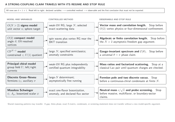
Representative $1+1$-dimensional laboratories answer different questions. The $O(N>2)$ model, $O(2)$ model, $\mathrm{CP}^{N-1}$ model, principal chiral model, discrete Gross–Neveu model, and massless one-flavor Schwinger model have different controls and observables. The schematic map forbids transferring a model-specific gap, topological, integrability, or screening conclusion to another theory without a new argument.

Strong-laboratory regime comparison

The table makes the same scope boundaries explicit in a form that does not depend on the figure. “Controlled method” names a limit or exact equivalence, not merely a calculational preference.

Variables, controls, observables, cross-checks, and forbidden extrapolations in representative strong-coupling laboratories.

Model and regime	Fields or variables	Symmetry or topology	Convention and limit order	Controlled method or limit	Physical observable	Independent cross-check	Scope boundary
O(N), N > 2, 1+1 dimensions	Unit vector n; auxiliary constraint field at large N	Global O(N); sphere target	Action normalized by 1/(2g²); hold t = Ng² at large N; require a/ξ → 0 and L/ξ → ∞	Weak-coupling RG, large N, and for selected cases exact scattering	Vector-channel mass and correlation length	Agreement among RG scaling, large-N saddle, exact data, and continuum lattice ratios	Does not include O(2) vortex physics or prove a four-dimensional confinement mechanism
O(2), 1+1 dimensions	Compact angle and vortices	U(1) rotations; integer vortex winding in Euclidean space	Declare stiffness and UV vortex-core regulator; take the thermodynamic limit before assigning a phase	Spin-wave and vortex renormalization group near the BKT transition	Algebraic or finite correlation length and vortex response	Universal jump and finite-size scaling in the corresponding statistical model	The O(N > 2) asymptotic-freedom and mass-gap argument does not apply
CP(N−1), 1+1 dimensions	Constrained complex z and emergent U(1) connection	Projective target; integer flux on closed Euclidean spacetime when bundle conditions hold	Hold t = Ng² at large N; declare bundle, θ, compactification, and volume before the infrared limit	Large N, semiclassics on specified compactifications, and anomaly constraints	Gauge-invariant spectrum and vacuum energy as a function of θ	Matching of topological periodicity, anomalies, and overlapping controlled regimes	No universal θ = π infrared phase may be inferred for all N and boundary conditions
SU(K) principal chiral model, 1+1 dimensions	Group-valued field U and left/right currents	SU(K)L × SU(K)R with diagonal stabilizer; classical nonlocal charges	Fix invariant-trace normalization and the line or circle boundary condition before defining monodromy	Weak-coupling RG plus separately established quantum integrability	Mass ratios and factorized scattering data	Yang–Baxter consistency, unitarity, crossing, bootstrap closure, and ultraviolet checks	A classical Lax connection alone does not establish a quantum S-matrix
Discrete Gross–Neveu, 1+1 dimensions	N Dirac fermions and auxiliary scalar σ	Discrete chiral symmetry; two large-N saddle vacua	Four-fermion term g²(ψ̄ψ)²/(2N); hold g² fixed and take infinite volume before diagnosing discrete breaking	Large N and asymptotically free perturbation theory	Fermion pole mass and gauge-invariant bilinear correlators	Gap equation, scattering data, and finite-N continuum calculations	Continuous-chiral variants obey different low-dimensional symmetry constraints
Massless one-flavor Schwinger model, 1+1 dimensions	Dirac fermion, U(1) gauge field, and bosonized scalar	Gauge symmetry and axial anomaly; electric-flux sectors depend on boundary data	D = ∂ − ieA; massless one-flavor infinite line in the zero-flux sector	Exact bosonization in a declared zero-flux sector	One neutral boson of mass e/√π and screened external-probe potential	Agreement of anomaly, current correlators, and bosonized equations	Massive fermions, multiple flavors, θ, and dynamical charged states change the conclusion

A control statement has four parts

A reliable strong-coupling result should identify:

1. the theory, including dimension, global form, boundary conditions, and normalization;
2. the controlled parameter or exact equivalence, such as $1/N$, weak ultraviolet coupling, a semiclassical compactification, or bosonization;
3. the observable actually computed, such as a gauge-invariant two-point function, vacuum energy, or static-probe potential;
4. the first omitted effect and the regime in which it is suppressed.

For example, a large-$N$ auxiliary saddle may generate a parameter $m$. Calling it “the mass” is justified only after a declared correlator has a pole or exponential decay at that value. In the $O(N)$ model this match occurs at leading order for the vector correlator; in $\mathrm{CP}^{N-1}$, the gauge-charged $z$ field is not by itself a physical asymptotic observable.

Common pitfalls

Inferring a phase from curvature. Ricci curvature controls perturbative metric running in a fixed convention. It does not by itself establish a mass gap, a unique vacuum, or confinement.

Treating every sigma model as ultraviolet complete. Above two dimensions the two-derivative action is normally an EFT. A cutoff and higher-derivative operators are part of the definition unless a separate fixed-point or microscopic construction is supplied.

Calling an auxiliary saddle a particle. A saddle parameter becomes a physical mass only through an observable correlator or finite-volume energy. Gauge redundancy, compositeness, and subleading corrections can change that translation.

Exercises

1. Expand the constrained $O(N)$ action about $n^N=\sqrt{1-\pi^i\pi^i}$ through quartic order in $\pi^i$, with $i=1,\ldots,N-1$. Identify the derivative interaction.

Solution

Since $\partial_\mu n^N=-(\pi\cdot\partial_\mu\pi)/\sqrt{1-\pi^2}$,

$$(\partial_\mu n)^2 =(\partial_\mu\pi)^2 +\frac{(\pi\cdot\partial_\mu\pi)^2}{1-\pi^2} =(\partial_\mu\pi)^2 +(\pi\cdot\partial_\mu\pi)^2 +O(\pi^6).$$

Thus

$$\mathcal L =\frac{1}{2g_0^2} \left[ (\partial_\mu\pi)^2 +(\pi\cdot\partial_\mu\pi)^2 +O(\pi^6) \right].$$

After canonically normalizing $\pi=g_0\varphi$, the quartic interaction is proportional to $g_0^2(\varphi\cdot\partial\varphi)^2$, displaying the loop-counting role of $g_0^2$.

2. Explain why the two-derivative sigma-model action is power-counting nonrenormalizable for $d>2$.

Solution

With dimensionless target coordinates, $[g_0^2]=2-d<0$. Expanding the target metric generates interactions with couplings of negative mass dimension. Loop divergences therefore require independent higher-derivative counterterms. Predictivity is recovered as an EFT expansion in $E/\Lambda_{\mathrm{EFT}}$, not by keeping only the two-derivative term at arbitrary energy.

Continue

Use The O(N) Model as a Strong-Coupling Laboratory for the sphere target and a controlled large-$N$ gap equation. The CP(N−1) Model adds a projective quotient, an emergent connection, and topological sectors. The Principal Chiral Model and the Integrability Bridge shows what extra evidence is required before classical conserved structures become exact quantum data.

References

• Friedan, Daniel. “Nonlinear Models in $2+\varepsilon$ Dimensions.” Physical Review Letters 45 (1980): 1057–1060. DOI.
• Friedan, Daniel H. “Nonlinear Models in $2+\varepsilon$ Dimensions.” Annals of Physics 163 (1985): 318–419. DOI.
• Polyakov, Alexander M. Gauge Fields and Strings. Contemporary Concepts in Physics 3. Harwood Academic Publishers, 1987, chs. 5–6. Publisher record.