Matrix Eigenvalue Saddles, Loop Equations, and Phase Transitions

An $N\times N$ Hermitian matrix integral becomes a continuum eigenvalue problem because diagonalization produces a Vandermonde determinant of order $N^2$. The normalized resolvent fixes the density through its branch-cut discontinuity, while the condition $W(z)\sim1/z$ fixes the endpoints. For the even quartic model solved below, positivity selects a one-cut phase for $r\ge-2\sqrt g$ and a symmetric two-cut phase for $r<-2\sqrt g$.

Required background. Large-N limits, normalizations, and orders of limits supplies the matrix action normalization, normalized trace, and fixed-coupling prescription.

Helpful background. Laurent series, poles, and residues supplies the large-$z$ matching and discontinuity calculation.

From the matrix measure to a density

Consider the convergent zero-dimensional integral

$$Z_N(r,g) = \int_{\mathrm{Herm}(N)}\mathrm dM\, \exp\!\left[-N\operatorname{tr}V(M)\right], \qquad V(x)=\frac r2x^2+\frac g4x^4, \qquad g>0.$$

The field is normalized exactly as on the scaling page: the action has an overall $N$, $r$ and $g$ are fixed as $N\to\infty$, and

$$\frac1N\operatorname{tr}M^k=O(1).$$

Diagonalize $M=U\,\mathrm{diag}(\lambda_1,\ldots,\lambda_N)U^\dagger$. After the angular integral,

$$Z_N \propto \int_{\mathbb R^N} \prod_{i=1}^N\mathrm d\lambda_i\, \exp\!\left[ -N\sum_iV(\lambda_i) +2\sum_{i<j}\log\lvert\lambda_i-\lambda_j\rvert \right].$$

The logarithm is eigenvalue repulsion. Varying one eigenvalue gives

$$V'(\lambda_i) = \frac2N\sum_{j\ne i} \frac1{\lambda_i-\lambda_j}.$$

Define the normalized empirical density and its limiting saddle by

$$\rho_N(x) = \frac1N\sum_{i=1}^N\delta(x-\lambda_i), \qquad \rho_N\longrightarrow\rho, \qquad \int_{\mathbb R}\mathrm dx\,\rho(x)=1.$$

At a regular point of the support,

$$V'(x) = 2\,\mathrm P \int\mathrm dy\,\frac{\rho(y)}{x-y}.$$

The continuum derivation and its $N^2$ effective action are given in Mariño 2015, §8.2, pp. 243–252.

Resolvent conditions and the one-cut solution

Define

$$W(z) = \int\mathrm dx\,\frac{\rho(x)}{z-x} = \frac1z+\frac{\langle x\rangle}{z^2} +\frac{\langle x^2\rangle}{z^3}+\cdots.$$

The coefficient of $1/z$ is exactly one because $\rho$ is normalized. Across a cut,

$$W(x+i0)+W(x-i0)=V'(x),$$

and

$$\rho(x) = -\frac{1}{2\pi i} \left[ W(x+i0)-W(x-i0) \right].$$

For an even one-cut solution supported on $[-a,a]$, choose the square root with

$$\sqrt{z^2-a^2}\sim z \qquad(z\to\infty).$$

Since $V'(z)=rz+gz^3$, the most general symmetric one-cut ansatz with the required discontinuity is

$$W_1(z) = \frac12 \left[ rz+gz^3 -\left(gz^2+c\right)\sqrt{z^2-a^2} \right].$$

Expanding at infinity,

$$\sqrt{z^2-a^2} = z-\frac{a^2}{2z}-\frac{a^4}{8z^3} +O(z^{-5}).$$

Cancellation of the term proportional to $z$ gives

$$c=r+\frac{ga^2}{2}.$$

Requiring the remaining $1/z$ coefficient to equal one gives

$$4ra^2+3ga^4=16.$$

The positive solution is

$$a^2 = \frac{2}{3g} \left( \sqrt{r^2+12g}-r \right).$$

Taking the discontinuity,

$$\rho_1(x) = \frac{1}{2\pi} \left(gx^2+c\right) \sqrt{a^2-x^2}, \qquad \lvert x\rvert\le a.$$

The same large-$z$ condition that fixed $a$ also proves normalization. It is not optional: a different resolvent branch can solve the cut equation while carrying the wrong total eigenvalue number.

Eigenvalue support and phase map

The figure freezes $g=1$ and shows three exact densities: $r=-1$ in the positive one-cut phase, $r=-2$ at the support-splitting boundary, and $r=-3$ in the symmetric two-cut phase. Inspect the origin. The one-cut density is positive there for $r>-2$, vanishes quadratically at $r=-2$, and is replaced by a gap for $r<-2$.

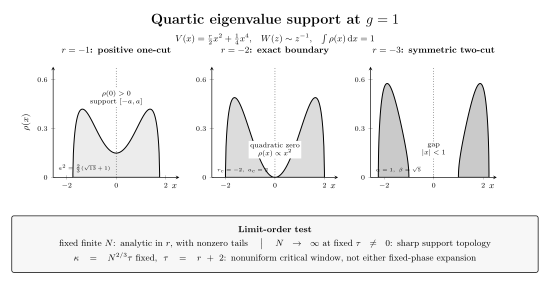
Normalized equilibrium densities for $V(x)=rx^2/2+x^4/4$ at $N=\infty$. The curves use the exact formulas on this page and are quantitative, with unit-normalized area. The phase boundary is $r_c=-2$; at every fixed finite $N$ the stable integral is analytic in $r$, so the sharp support topology and any critical scaling window belong to specified large-$N$ limits rather than a finite-$N$ singularity.

The map encodes a positivity test as well as an algebraic solution. A formally normalized density that is negative anywhere is not an equilibrium measure.

Positivity and the two-cut phase

For $g>0$, the polynomial $gx^2+c$ is smallest at the origin. The one-cut density is nonnegative precisely when

$$c = r+\frac{ga^2}{2} \ge0.$$

At the boundary $c=0$. Combining this with the normalization equation gives

$$r_c=-2\sqrt g, \qquad a_c^2=\frac4{\sqrt g}.$$

For $r<-2\sqrt g$, the one-cut formula is negative near $x=0$ and must be rejected. The symmetric equilibrium measure instead has support

$$[-\beta,-\alpha]\cup[\alpha,\beta],$$

where

$$\alpha^2 = \frac{-r-2\sqrt g}{g}, \qquad \beta^2 = \frac{-r+2\sqrt g}{g}.$$

Its density is

$$\rho_2(x) = \frac{g\lvert x\rvert}{2\pi} \sqrt{(x^2-\alpha^2)(\beta^2-x^2)}$$

on the two intervals and zero outside. Its normalization can be checked without a resolvent:

$$\begin{aligned} \int\mathrm dx\,\rho_2(x) &= \frac{g}{2\pi} \int_{\alpha^2}^{\beta^2}\mathrm du\, \sqrt{(u-\alpha^2)(\beta^2-u)}\\ &= \frac{g}{16} \left(\beta^2-\alpha^2\right)^2 =1. \end{aligned}$$

At $r=r_c$, $\alpha\to0$, $\beta^2\to4/\sqrt g$, and $\rho_2$ joins the critical one-cut density. The even potential selects equal filling of the two wells in the symmetric equilibrium problem. A constrained unequal filling is different boundary data.

This solution is a direct instance of the planar eigenvalue and loop-equation method developed in Brézin et al. 1978, pp. 37–45.

Loop equation and branch rejection

At finite $N$, integration by parts produces a loop equation for

$$W_N(z) = \frac1N \left\langle \operatorname{tr}\frac1{z-M} \right\rangle.$$

Its planar part has the algebraic form

$$W(z)^2-V'(z)W(z)+P(z)=0,$$

where $P$ is fixed by moments and asymptotics. The quadratic equation has two formal branches. Only the branch with

$$W(z)\sim\frac1z, \qquad \rho(x)\ge0, \qquad \int\mathrm dx\,\rho(x)=1$$

is admissible for the declared saddle. Additional cuts require filling-fraction conditions; the polynomial equation alone does not choose them. The resolvent’s analytic and asymptotic characterization is summarized in Mariño 2015, §8.2, pp. 252–258.

The parameter and N limits

For $g>0$ and finite $N$, $Z_N(r,g)$ and its finite moments are analytic for real $r$. There is no exact finite-$N$ compact support: eigenvalue tails are small but nonzero. The sharp statements

$$\operatorname{supp}\rho = \begin{cases} [-a,a], & r>-2\sqrt g,\\ [-\beta,-\alpha]\cup[\alpha,\beta], & r<-2\sqrt g \end{cases}$$

refer to the equilibrium density obtained after $N\to\infty$ at fixed nonzero $r-r_c$.

Approaching $r_c$ while $N$ grows probes a separate critical window. Fixed one-cut or two-cut $1/N$ coefficients become nonuniform there, and a double-scaled description is required. Thus the operations “take $N\to\infty$ at fixed phase” and “approach the phase boundary within an $N$-dependent window” are not interchangeable. Rigorous quartic-matrix asymptotics distinguish regular one-cut expansions from the singular double-scaling regime Bleher and Its 2005, §§1–2.

Shared comparison. The large-N scaling comparison fixes the matrix action, operator normalization, and critical-limit warning used here.

Common pitfalls

Keeping a normalized but negative one-cut density. Normalization is necessary, not sufficient. At $r<-2\sqrt g$, positivity forces a change of support.

Choosing the other algebraic resolvent branch. The saddle equation alone leaves a quadratic ambiguity. The physical branch has $W(z)\sim1/z$ and a nonnegative normalized discontinuity.

Calling the finite-N crossover a phase transition. The sharp support topology belongs to the limiting density. State how $r-r_c$ scales with $N$ before using critical asymptotics.

Exercises

1. Derive the discrete saddle equation from the eigenvalue integral.

Solution

The negative logarithm of the integrand is

$$S_{\mathrm{eig}} = N\sum_iV(\lambda_i) -2\sum_{i<j}\log\lvert\lambda_i-\lambda_j\rvert.$$

Setting $\partial S_{\mathrm{eig}}/\partial\lambda_i=0$ gives

$$NV'(\lambda_i) -2\sum_{j\ne i}\frac1{\lambda_i-\lambda_j} =0,$$

which yields the stated equation after division by $N$.

2. Expand $W_1(z)$ through order $1/z$ and recover the equations for $c$ and $a$.

Solution

Using

$$(gz^2+c)\sqrt{z^2-a^2} = gz^3 +\left(c-\frac{ga^2}{2}\right)z -\left(\frac{ca^2}{2}+\frac{ga^4}{8}\right)\frac1z +\cdots,$$

cancellation of the $z$ term gives $c=r+ga^2/2$. The $1/z$ coefficient of $W_1$ is $ca^2/4+ga^4/16$. Setting it to one gives $4ra^2+3ga^4=16$.

3. Show that the one-cut positivity boundary is $r=-2\sqrt g$.

Solution

At the boundary, $c=r+ga^2/2=0$, so $r=-ga^2/2$. Insert this into

$$4ra^2+3ga^4=16$$

to obtain $ga^4=16$. Thus $a^2=4/\sqrt g$ and $r=-2\sqrt g$.

4. Normalize the two-cut density by substituting $u=x^2$.

Solution

Evenness gives

$$\begin{aligned} \int\mathrm dx\,\rho_2(x) &= \frac g\pi \int_\alpha^\beta\mathrm dx\,x \sqrt{(x^2-\alpha^2)(\beta^2-x^2)}\\ &= \frac{g}{2\pi} \int_{\alpha^2}^{\beta^2}\mathrm du\, \sqrt{(u-\alpha^2)(\beta^2-u)}. \end{aligned}$$

The last integral equals $\pi(\beta^2-\alpha^2)^2/8$. Since $\beta^2-\alpha^2=4/\sqrt g$, the result is one.

References

• Bleher, P. M., and Its, A. R. (2005). “Asymptotics of the Partition Function of a Random Matrix Model.” Annales de l’Institut Fourier 55, 1943–2000. doi:10.5802/aif.2147. Open PDF.
• Brézin, E., Itzykson, C., Parisi, G., and Zuber, J.-B. (1978). “Planar Diagrams.” Communications in Mathematical Physics 59, 35–51. doi:10.1007/BF01614153.
• Mariño, M. (2015). Instantons and Large N: An Introduction to Non-Perturbative Methods in Quantum Field Theory. Cambridge University Press. doi:10.1017/CBO9781107705968.