Finite-Energy Boundary Data, Charge, and Stability

A finite-energy boundary condition does more than control a field’s tail: it specifies the configuration space in which topology can be discussed. For a defect of codimension $c$, the fields on a large transverse sphere $S^{c-1}_\infty$ must approach the vacuum data, so a configuration may define a homotopy class of maps into the physical vacuum manifold. Distinct classes cannot be connected by a continuous finite-energy path. This classifies sectors; it does not by itself prove that a smooth solution exists, that an energy infimum is attained, or that the solution is dynamically or quantum mechanically stable.

Required background. Homotopy, degree, and winding supplies the classification of maps, while vacuum orbits and unbroken subgroups identifies the physical vacuum manifold. Helpful background. Classical symmetries and variational field equations explains the energy functional and its stationary points.

Finite energy fixes the admissible boundary maps

Let $D$ be the number of spatial dimensions, and consider a static defect extended along $D-c$ directions. Its transverse space is $\mathbb R^c$. Assume the fields are regular and their asymptotic limits are uniform enough for the energy integrals and integrations by parts below to exist. For canonical scalar and gauge kinetic terms, finite energy per unit defect volume then requires, schematically,

$$D_i\phi\longrightarrow 0,\qquad V(\phi)\longrightarrow V_{\min},\qquad F_{ij}\longrightarrow 0 \quad\text{as }r_\perp\longrightarrow\infty .$$

These conditions determine which boundary data are admissible. In a global theory with vacuum manifold $\mathcal M$, the asymptotic scalar field defines

$$\phi_\infty:S^{c-1}_\infty\longrightarrow\mathcal M .$$

Without a chosen base point, the homotopy datum is the free-homotopy set $[S^{c-1},\mathcal M]$. Identifying it with the based group $\pi_{c-1}(\mathcal M)$ requires a reference vacuum and, when relevant, accounting for the action of $\pi_1(\mathcal M)$. For $c=1$, $S^0_\infty$ consists of two points, so the complete datum is the ordered pair of endpoint components rather than one group element. Boundaries, interfaces, prescribed defects, or nontrivial bundles can instead require relative homotopy.

In a gauge theory, one must quotient only by gauge transformations declared redundant at infinity; transformations acting nontrivially on boundary data can label physical charges rather than redundancies. The global form of the gauge group and the allowed matter representations therefore matter.

For a local gauge defect, the asymptotic field–connection pair cannot in general be replaced by an ordinary map into the fully gauge-quotiented vacuum space. In the Abelian Higgs model that quotient is a point, yet the allowed Higgs trivialization and connection at infinity retain an integer winding and flux class. Which transformations are permitted at infinity, together with the bundle and charge lattice, is part of the configuration space being classified.

The transverse-sphere rule is the organizing idea behind the family map below. Inspect which sphere supplies the boundary domain and whether the classification uses a vacuum map, gauge-boundary or bundle data, or the compactified whole space.

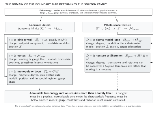
Boundary data classify different soliton families in different ways. A codimension-$c$ defect uses $S^{c-1}_\infty$; a texture or lump commonly uses the one-point compactification of all space. The diagram is schematic: existence, stability, and the dimension of the moduli space still require a model-specific analysis.

Swipe horizontally to inspect the complete classification, or open the vector figure at full size.

The same information in compact form is:

• a wall or kink samples two ends of a transverse line, $S^0_\infty$, and can distinguish disconnected vacua;
• a vortex samples a circle around its core and can carry winding or gauge flux;
• a smooth monopole samples a two-sphere at infinity and combines a Higgs-direction map with an asymptotic Abelian magnetic field;
• a lump or Skyrmion maps compactified whole space into its target, so its charge is not obtained by blindly applying the defect codimension rule.

This separation between boundary classification and field equations is emphasized in Coleman 1985, § 3, pp. 195–222 and developed systematically in Manton and Sutcliffe 2004, §§ 3.1–4.2, pp. 47–86.

The kink sector as a complete boundary calculation

Consider a real scalar in $1+1$ dimensions,

$$\mathcal L =\frac12\partial_\mu\phi\,\partial^\mu\phi -\frac{\lambda}{4}\left(\phi^2-v^2\right)^2, \qquad \lambda>0,\quad v>0 .$$

For a static configuration on $\mathbb R$,

$$E[\phi] =\int_{-\infty}^{\infty}\mathrm dx \left[ \frac12(\phi')^2 +\frac{\lambda}{4}\left(\phi^2-v^2\right)^2 \right].$$

Finite energy requires $\phi(\pm\infty)\in\{-v,+v\}$. The boundary pair is a map from $S^0_\infty=\{-\infty,+\infty\}$ to the two-point vacuum manifold. With an orientation on the spatial line, define

$$Q_{\mathrm K} =\frac{\phi(+\infty)-\phi(-\infty)}{2v}.$$

Then $Q_{\mathrm K}=+1$ for a kink, $-1$ for an antikink, and $0$ when the two endpoints agree. The single number is not the complete $S^0$ datum: $(+v,+v)$ and $(-v,-v)$ both have $Q_{\mathrm K}=0$ but remain different endpoint pairs unless a global symmetry is also quotiented. A continuous finite-energy deformation cannot change either endpoint without passing through nonvacuum values over an unbounded region or losing the boundary limit. This establishes sector separation.

It still does not construct a kink. Existence follows here because the energy can be completed into a square and the resulting first-order equation has the smooth solution

$$\phi_{\mathrm K}(x) =v\tanh\!\left[\frac{m}{2}(x-X)\right], \qquad m^2=2\lambda v^2 ,$$

where $X$ is the translation modulus. The construction and the fluctuation test belong to Kinks and Domain Walls. The boundary calculation remains valid independently of that explicit profile.

Five logically different stability questions

A precise claim should pass through five separate questions.

1. Sector: do the declared boundary conditions define disconnected components of the admissible configuration space?
2. Existence: does the energy have a stationary point in the chosen sector, and is the relevant infimum attained rather than approached by shrinking, spreading, or escaping to infinity?
3. Energetic stability: is the solution a local or absolute minimum under the allowed variations, possibly at fixed charge?
4. Dynamical stability: does the linearized operator have negative modes, and does nonlinear time evolution remain close to the symmetry orbit of the solution?
5. Quantum survival: after renormalization and tunneling channels are included, is there a stable state, a resonance with a calculable width, or no identifiable excitation?

These implications do not reverse. Nontrivial homotopy can obstruct decay to the vacuum while allowing a configuration to shrink without a smooth minimizer. A nonnegative quadratic fluctuation operator is only a linear statement and may contain zero modes that require collective coordinates. A classical minimum need not be protected against quantum decay if the exact theory permits a channel not visible in the classical truncation.

The stability diagram makes the required test explicit for each common mechanism. Read each row from the construction on the left to the statement that is actually justified on the right.

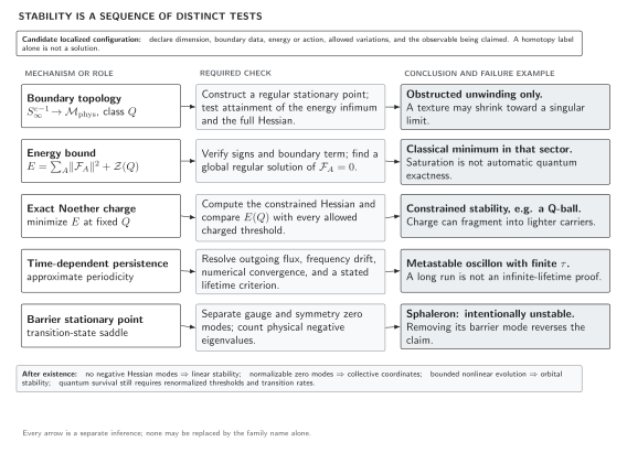
Localized configurations are not all stable for the same reason. Topology labels sectors, an energy bound controls a variational problem, fixed charge defines a constrained minimum, an oscillon has a finite dynamical lifetime, and a sphaleron is intentionally unstable. The diagram is schematic and does not assert existence for any model.

Swipe horizontally to inspect every inference test, or open the vector figure at full size.

Soliton boundary and stability comparison

The table is a semantic counterpart to the diagrams and a compact check against category errors. Its construction, virial, fluctuation, and scope columns keep sector classification, classical stability, lifetime, and quantum survival logically separate.

Boundary data, charges, stability claims, and known failure modes for representative localized configurations.

Family	Boundary data and charge or constraint	Existence or construction	Virial test or energy bound	Fluctuation and classical status	Moduli or lifetime	Quantum or scope boundary
Kink / wall	Codimension 1; the ordered endpoint components lie in disconnected vacua; a scalar kink charge is model- and convention-dependent	Explicit ODE solution or a variational existence argument with fixed endpoints	E₂ = E₀; a smooth square-completion function W can give T ≥ |ΔW|	The φ⁴ kink has no negative mode and is a minimum in its fixed boundary sector	Position; sometimes an exact internal orientation	Disconnected vacua do not construct a wall; renormalized mass and decay channels need a quantum calculation
Local vortex	Codimension 2; a circle at infinity has covariantly constant Higgs data; flux is tied to winding and the charge lattice	Regular elliptic or radial profile with a resolved scalar and magnetic core	Gauge and Higgs terms evade scalar scaling; for λ ≥ e², T ≥ 2πv²|n|, with equality only at λ = e² for a nontrivial vortex	Stability depends on winding and coupling; critical vortices have a nonnegative physical Hessian with positional zero modes	Transverse positions at critical coupling; internal orientations in extended models	A global vortex has logarithmically divergent infinite-volume tension; flux alone does not settle quantum string stability
Smooth monopole / dyon	Codimension 3; the Higgs direction maps the sphere at infinity into G/H; magnetic charge and possible dyonic electric data	Smooth gauge–Higgs field equations with a resolved non-Abelian core	Gauge fields change the scaling; for a nonnegative Higgs potential, M ≥ 4πv|nₘ|/g, with equality only in the Prasad–Sommerfield limit	BPS saturation gives a nonnegative physical Hessian; away from it the spectrum is model-dependent	Position and electric phase in the BPS regime; relative data for multiple monopoles	Dirac boundary data do not supply a smooth core, and quantum BPS exactness needs additional supersymmetry
Sigma-model lump	Two-dimensional whole space compactifies to a sphere; charge is the degree of the target-space map	Holomorphic or antiholomorphic rational map in the two-derivative O(3) model	Scale invariant; E ≥ 4π|Q|/g²	A saturated fixed-degree minimum has a flat scale direction rather than a restoring force	Position, scale, and target orientation; some kinetic norms can diverge on the infinite plane	Running or perturbations can lift the scale and drive collapse or spreading; the classical bound is not quantum protection
Skyrmion	Three-dimensional whole space compactifies to a sphere and maps into the group target; degree is conventionally baryon number	Regular nonlinear variational solution, usually with a numerically determined profile	E₂ = E₄ in the massless model; no generic saturated first-order bound	The dilation direction is positive at the virial balance, but the full Hessian is still required	Position and spatial/internal orientation; size is fixed, not a modulus	Topology does not fix size; EFT truncation, global quantization constraints, and loop corrections remain separate
Q-ball	Fields approach one vacuum at infinity; the exact constraint is a fixed global Noether charge	Constrained radial profile in a potential admitting a nonempty frequency interval	Extremize E − ωQ; there is no topological first-order bound	A stable branch requires a nonnegative fixed-Q Hessian and comparison with fragmentation channels	Position and global phase	Charge prevents disappearance but not decay into a lower-energy collection of charged states
Oscillon	Localized approximately periodic field with vacuum tails; no exact charge generically	Converged real-time evolution or a controlled asymptotic construction	Static Derrick scaling does not apply to the motion; no generic energy bound	Metastable persistence is determined by outgoing radiation and frequency drift	Finite lifetime τ; center, phase, amplitude, and frequency are only approximate collective data	A finite simulation gives a lower bound on lifetime, not an exact breather or a quantum decay rate
Sphaleron	Barrier-top configuration between sectors or vacua; the barrier coordinate is not a protecting charge	Regular stationary solution on a declared transition path	Stationarity may satisfy a virial relation, but there is no protecting lower bound	A physical negative mode makes it a saddle; index one is common on a minimal barrier path	Symmetry zero modes only after the negative direction is separated	Calling it stable reverses its role; its energy alone is neither a tunneling nor a thermal transition rate

The nontopological rows use three different kinds of primary evidence: Coleman’s fixed-charge variational construction for Q-balls Coleman 1985, pp. 263–283, the small-amplitude radiation obstruction for generic $\phi^4$ breathers Segur and Kruskal 1987, pp. 747–750, and the electroweak barrier saddle Klinkhamer and Manton 1984, pp. 2212–2220. These sources support the distinct fixed-charge, finite-lifetime, and negative-mode claims; none turns one category into another.

What topology can and cannot establish

Topology is strongest as a statement about paths in configuration space. It can show that a finite-energy evolution preserving the boundary conditions cannot unwind a charge. It can also supply a lower bound when the energy admits an appropriate inequality. Neither statement guarantees a smooth minimizer: compactness, regularity, gauge fixing, and the possibility of concentration or escape still matter.

Conversely, a configuration need not carry a topological charge to persist. A Q-ball can minimize energy at fixed Noether charge, an oscillon can radiate extremely slowly, and a sphaleron can organize transitions precisely because it has an unstable direction. Manton and Sutcliffe 2004, §§ 4.1–4.5, pp. 75–108 give the general topology, scaling, and moduli framework; the following pages test each mechanism in a concrete model.

Common pitfalls

Using homotopy as an existence theorem. A nonzero homotopy class says that admissible maps cannot be continuously unwound. One must still solve or control the variational problem and show that the putative minimum does not collapse, spread, or develop a singularity.

Quotienting the wrong transformations at infinity. A gauge transformation that changes permitted boundary data may act as a physical global symmetry. The gauge group’s global form, matter charge lattice, and allowed asymptotic transformations must be stated before assigning a charge.

Calling every persistent object topological. Fixed-charge minima, metastable oscillations, and barrier saddles have different observables and failure modes. The relevant test is respectively constrained energy, lifetime under evolution, or fluctuation index.

Exercises

1. For the $\phi^4$ model above, show that $Q_{\mathrm K}$ is invariant under any continuous one-parameter family $\phi_s(x)$ whose endpoint limits remain in $\{-v,+v\}$.

Solution

For each endpoint, $s\mapsto\phi_s(\pm\infty)$ is a continuous map from a connected interval into the discrete set $\{-v,+v\}$. It is therefore constant. Their normalized difference $Q_{\mathrm K}$ is constant as well. The argument fails if an endpoint limit ceases to exist or leaves the vacuum set, which is exactly where the finite-energy configuration space has been left.

2. A three-dimensional scalar theory has vacuum manifold $S^2$. A point-defect boundary map may have nonzero degree in $\pi_2(S^2)$. Explain why this alone does not contradict Derrick’s obstruction for an energy containing only two-derivative gradient and nonnegative potential terms.

Solution

The homotopy class constrains boundary-preserving paths but does not ensure that the energy infimum is achieved by a smooth finite-size configuration. With canonical two-derivative gradients, a nonconstant map on every large sphere also produces the familiar linearly divergent global-monopole energy, so the premise need not even define a finite-total-energy sector. If the infrared behavior is otherwise regulated, spatial rescaling still prevents nonnegative two-derivative and potential terms from satisfying the three-dimensional stationary virial relation. Gauge fields, higher derivatives, or a changed geometry are needed before a smooth finite-size object can evade these obstructions.

3. In the Abelian Higgs model, the fully gauge-quotiented vacuum space is a point. Why can the theory nevertheless have integer vortex sectors?

Solution

The quotient of constant vacuum field values does not retain the full asymptotic field–connection data. Finite energy requires a covariantly constant Higgs field on $S^1_\infty$, and its phase winding is tied to the gauge connection through $D_\theta\phi\to0$. Once the allowed gauge transformations at infinity and the charge lattice are fixed, the resulting holonomy or bundle class gives

$$\frac{e}{2\pi}\int_{\mathbb R^2}F\in\mathbb Z .$$

Thus the integer belongs to the admissible gauge configuration and its boundary trivialization, not to $\pi_1$ of a one-point vacuum quotient.

Continue

Use Derrick Scaling, Virial Tests, and Nontopological Stability to test whether an energy can support a finite size. Then choose a family: kinks, vortices, monopoles, or lumps and Skyrmions.

References

• Coleman, Sidney. Aspects of Symmetry: Selected Erice Lectures. Cambridge University Press, 1985, ch. 6, “Classical Lumps and Their Quantum Descendants,” pp. 185–264. DOI.
• Coleman, Sidney. “Q-Balls.” Nuclear Physics B 262 (1985): 263–283; erratum 269 (1986): 744. Article DOI; erratum DOI.
• Klinkhamer, Frans R., and Nicholas S. Manton. “A Saddle-Point Solution in the Weinberg–Salam Theory.” Physical Review D 30 (1984): 2212–2220. DOI.
• Manton, Nicholas, and Paul Sutcliffe. Topological Solitons. Cambridge Monographs on Mathematical Physics. Cambridge University Press, 2004, chs. 3–4. DOI.
• Segur, Harvey, and Martin D. Kruskal. “Nonexistence of Small-Amplitude Breather Solutions in $\phi^4$ Theory.” Physical Review Letters 58 (1987): 747–750. DOI.