Claim Status Across Nonperturbative Methods

A nonperturbative claim should be labeled proposition by proposition, not method by method. An exact identity can feed an uncontrolled closure; a regulated computation can support a continuum conclusion only through explicit extrapolations; an exact S matrix can remain conditional on completeness and locality; and many mutually consistent calculations can coexist with an open construction problem. The appropriate label is therefore the strongest one justified for the precise observable, hypotheses, limits, and inference being asserted—and no stronger.

Required background. What “nonperturbative” means in a declared problem supplies the control-first vocabulary. Confinement evidence and open problems, evidence and limits for resurgence, and functional-method validation supply three deliberately different test cases.

Helpful background. Renormalized saddle contributions and validity tests gives a compact example in which a controlled asymptotic statement, a numerical check, and an exact spectral observable must remain distinct.

Shared framework. The method–evidence map separates a method from its control and evidence status, while the claim-and-control comparison supplies representative falsifiers.

Evidence classes attach to propositions

Begin by writing one proposition in a form that could be false:

In theory $T$, with state and boundary data $B$, the renormalized observable $O$ has property $P$ after limits $L_1,L_2,\ldots$ are taken in the stated order.

Then separate the ingredients supporting it. The following classes answer different questions.

• A definition fixes what the object means. It can be exact without showing that the object exists in the intended continuum theory.
• An exact identity follows from declared structural assumptions, such as a Ward identity or an anomaly relation. It constrains solutions but need not select one.
• A theorem proves a stated conclusion from explicit hypotheses. Its force does not extend to a different dimension, topology, regulator limit, or observable.
• A constructive result supplies the theory or observable as a mathematical object and controls the required cutoff and volume limits. Construction of one model does not construct a nearby model.
• A controlled approximation has a parameter or hierarchy that bounds, estimates, or systematically orders omitted effects in a specified regime.
• A regulated numerical result computes a finite-cutoff, finite-volume, or discretized quantity with numerical and systematic uncertainties. A continuum claim additionally requires a matching and limit argument.
• A phenomenological inference connects the theory calculation to measured or model-dependent inputs. It can be compelling while remaining conditional on that connection.
• A conjecture is a precise proposed statement not established by the available arguments. An open problem also names the missing construction, proof, or calculation.

These labels form neither a prestige ranking nor a single numerical scale. A theorem about a bound may answer less of a phenomenological question than a controlled computation of the observable, while the theorem remains logically stronger within its scope. Record instead the tuple

$$\mathcal C =\bigl(T,B,O,P;\,\text{hypotheses};\,\text{limits};\, \text{support};\,\text{uncertainty};\,\text{falsifier}\bigr).$$

Two statements receive the same status only if the relevant entries of this tuple agree.

Evidence triangulation graph

Agreement becomes informative only after every output has been translated to the same observable and shared inputs have been exposed. In the graph below, arrows mean depends on, not “confirms with this much weight.” Inspect especially the central shared-input node: the two upper methods do not become independent merely because their algorithms differ.

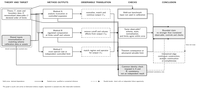
Evidence must be combined through a directed dependency graph. Shared renormalization, matching, ansätze, or calibration data merge upstream; method outputs are compared only after observable translation; and unresolved continuation or limit steps remain visible. The graph is schematic and assigns no numerical evidence weights.

The same graph as an adjacency list is:

1. the theory definition, state, observable, and limit order feed every method;
2. shared renormalization or matching input feeds both the analytic truncation and the regulated computation;
3. shared calibration data feed any ansatz or fit trained on those data;
4. each method output passes through its own normalization, continuation, and limit map before reaching the common observable;
5. a common identity check tests consistency but is not an independent determination if that identity was imposed in every method;
6. a held-out benchmark and a theorem consequence can supply genuinely different failure opportunities when their inputs are independent; and
7. the final node states only the conclusion supported after unresolved edges are retained.

A cycle would mean that a result is being used, directly or indirectly, to validate itself. For example, fitting a functional vertex to a lattice propagator and then presenting agreement of the resulting propagator with the same lattice data is calibration closure, not a new cross-method test.

Exact and rigorous status comparison

The comparison below is a semantic counterpart to the graph. “Exact” always modifies an object under stated assumptions; it is never shorthand for “the entire physical interpretation is proved.” Time-sensitive entries carry an explicit source cutoff.

Exact objects, controlled calculations, constructions, evidence, and open limits in representative nonperturbative claims

Model or claim	Exact object	Theorem or calculation	Essential hypotheses	Cutoff and volume status	Justified status	Open limit or inference	Status source or cutoff
Anomaly constraint on infrared behavior	Background-field variation or anomaly class	Exact matching obstruction under renormalization-group flow	Correct global symmetry, global form, allowed backgrounds, counterterms, and boundary conditions	Conditional on existence of the ultraviolet and infrared descriptions used	Exact structural constraint within the declared theory	Which compatible infrared realization dynamics selects	Evergreen statement; theory-specific status belongs with the model
Weak-coupling instanton contribution	Specified Euclidean boundary problem and observable	Saddle action, collective measure, determinant, and asymptotic corrections	Correct integration cycle, weak coupling at the saddle scale, controlled zero modes, renormalization, and dilute or isolated-event regime	Regulator removal and infrared size or volume limits must be checked for the model	Controlled asymptotic result where its hierarchy holds	Strong-coupling continuation or an uncontrolled size integral	Evergreen method statement
Compact Abelian confinement mechanism in three Euclidean dimensions	Dual compact scalar and its monopole-induced potential in the controlled effective theory	Dilute-gas dualization, dual-photon mass, and Wilson-loop domain wall	Compact gauge field, specified ultraviolet realization, weak monopole fugacity, and scale separation	Controlled within the stated regulated or ultraviolet-completed model and limit	Controlled mechanism in that regime	Transfer to noncompact QED or four-dimensional non-Abelian Yang–Mills	Evergreen scope statement
Factorized scattering in a two-dimensional integrable model	Candidate S matrix, finite-volume spectrum, or form factors	Unitarity, crossing, Yang–Baxter, bootstrap, Bethe, or thermodynamic-Bethe-ansatz calculation	Integrability, particle content, analyticity, physical-sheet convention, CDD choice, and locality assumptions	Often formulated directly in the continuum and infinite volume; finite-size reconstruction adds its own limits	Exact data conditional on the accepted model and completeness assumptions	Constructive realization, completeness, or uniqueness when not separately proved	Evergreen method statement
Interacting P(φ)₂ and selected φ⁴₃ models	Schwinger functions, Hilbert space, fields, and Hamiltonian in the constructed model	Constructive existence, cutoff removal, and reconstruction theorems	Specific spacetime dimension, stable renormalized interaction, and the hypotheses of the construction	Ultraviolet and infinite-volume limits controlled for the particular constructed models	Rigorous nonperturbative construction	Extension to a different interaction or four-dimensional gauge theory	Glimm–Jaffe constructive results; evergreen
Four-dimensional lattice Yang–Mills spectrum	Finite-spacing, finite-volume transfer-matrix levels and extrapolated gauge-invariant masses	Regulated simulation with continuum, volume, sampling, scale-setting, and operator-basis studies	Declared lattice action, gauge group, observables, estimators, and extrapolation models	Evidence depends on demonstrated continuum and infinite-volume stability over the simulated range	Regulated numerical evidence for the physical spectrum	Axiomatic continuum construction and a proved positive gap uniform in volume	Claim-specific dated computational dossier required
Four-dimensional quantum Yang–Mills existence and mass gap	A nontrivial axiomatic theory on R⁴ with spectral gap Δ greater than zero	No accepted proof of the stated construction and gap	Any compact simple gauge group and axiomatic properties at least as strong as the official statement requires	A finite regulator or box is not the requested conclusion	Open mathematical problem	Continuum existence and a positive infinite-volume mass gap	Clay Mathematics Institute status checked 9 August 2026

Osterwalder–Schrader reconstruction illustrates why “Euclidean data” and “a relativistic QFT” are not interchangeable labels: Euclidean covariance, reflection positivity, symmetry, regularity, and clustering or related conditions perform essential work in the reconstruction Osterwalder and Schrader 1973, pp. 83–112. Constructive models satisfy such requirements in specific dimensions and interactions; Glimm and Jaffe develop the cutoff removal and reconstruction program in detail Glimm and Jaffe 1987, chs. 6–19, pp. 157–456.

Decomposing a non-Abelian mass-gap claim

Consider the statement “four-dimensional pure Yang–Mills theory has a mass gap.” It contains at least four different propositions.

1. Definition: a physical gap is a positive lower edge of the spectrum above the vacuum in the gauge-invariant Hilbert space, equivalently reflected in exponential clustering under suitable reconstruction hypotheses.
2. Regulated result: finite lattice spacing and volume define a transfer-matrix or Euclidean spectral problem from which gauge-invariant energy levels can be estimated.
3. Translation and limits: those levels must be matched to a renormalized observable and shown stable as the operator basis, lattice spacing, spatial volume, and fitting window are varied.
4. Construction and theorem: the continuum theory must exist with the required axioms, and the positive gap must persist uniformly in the infinite-volume limit.

The first is a definition, the second and third can yield strong regulated numerical evidence, and the fourth remains the official open problem. The Clay Mathematics Institute’s statement explicitly asks for a nontrivial quantum Yang–Mills theory on $\mathbb R^4$ with $\Delta>0$ and reports that no proof is known Jaffe and Witten 2000, official problem description, pp. 129–152. Numerical evidence cannot be promoted into that proof by accumulation, because the missing conclusion is precisely control of the continuum construction and uniform limit.

The comparison with controlled models sharpens the distinction. In the large-$N$ two-dimensional O($N$) model, a saddle produces a gap with a systematic $1/N$ expansion, but this is not the finite-$N$ four-dimensional gauge theorem. In compact three-dimensional electrodynamics, a dilute monopole ensemble can yield a controlled dual-photon mass and area law, but compactness, dimension, and scale separation are indispensable hypotheses. These examples strengthen understanding of mechanisms; they do not prove a different theory.

How a claim changes status

A claim changes status only when the missing implication is supplied. Useful upgrade questions are:

• Has the same renormalized observable been computed, or only a proxy with a similar name?
• Was a parameter varied so that the first omitted effect became visible and followed the predicted scaling?
• Were continuum, volume, infrared, and large-parameter limits varied independently enough to test their order?
• Does the new comparison use independent inputs, or reuse the same calibration, ansatz, configurations, or matching coefficient?
• Has a theorem’s complete hypothesis set been verified for the physical model?
• What observation, counterexample, residual, or failed limit would lower the stated status?

The observable-translation workflow answers the first three questions, and the correlated-evidence analysis answers the fourth. Rigorous status and open problems develops the theorem and construction handoff. Dated changes in method reach or numerical evidence belong in the Nonperturbative Gauge Dynamics research guide, not in an undated generalization here.

Common pitfalls

Calling an identity an exact solution. A Schwinger–Dyson or Ward identity is exact, but a chosen closure and branch need separate control. Label each link rather than transferring “exact” to the output.

Treating continuum notation as continuum construction. Writing a formal functional integral on $\mathbb R^4$ does not establish that its regulator can be removed with the desired axioms. The limit itself is part of the claim.

Using agreement as proof of independence. Two methods can agree because they share the same ansatz or calibration data. Expose the common ancestors before judging what the agreement adds.

Exercises

Decompose the statement “an anomaly proves symmetry breaking” into an exact premise, an excluded infrared possibility, and the remaining dynamical alternatives.

Solution

The exact premise is the nontrivial anomaly class after the symmetry, global form, backgrounds, and allowed counterterms are fixed. Matching excludes an infrared theory that is simultaneously unique, trivially gapped, symmetry preserving, and without the required topological or gapless response. The remaining compatible possibilities can include spontaneous breaking, gapless degrees of freedom, topological order, an extended-operator response, or a boundary inflow realization. Choosing among them requires dynamics beyond the anomaly.

A regulated calculation reports a mass $aM=0.21(1)$ on three lattice spacings and two volumes. List the additional information required before calling it an infinite-volume continuum mass.

Solution

One needs the action and operator definition; scale setting and renormalization; autocorrelation and estimator uncertainties; an operator-basis and excited-state analysis; a continuum extrapolation justified over a resolved scaling range; a finite-volume study tied to the lightest relevant state; and the order in which the limits are taken. The quoted statistical uncertainty alone covers none of these systematic translations.

References

• Glimm, James, and Arthur Jaffe. Quantum Physics: A Functional Integral Point of View. 2nd ed. New York: Springer, 1987. DOI.
• Jaffe, Arthur, and Edward Witten. “Quantum Yang–Mills Theory.” In The Millennium Prize Problems, 129–152. Providence, RI: American Mathematical Society and Clay Mathematics Institute, 2006. Official PDF. Current official status.
• Osterwalder, Konrad, and Robert Schrader. “Axioms for Euclidean Green’s Functions.” Communications in Mathematical Physics 31, no. 2 (1973): 83–112. DOI. Open PDF.