Correlated Standard Model Fits and Consistency Tests

A correlated Standard Model fit is a specified joint probability model for exact input releases, shared parameters, shared nuisances, and any dataset overlap. It is not a sum of independently quoted pulls. Reliable consistency statements require a frozen validity domain, a calibrated test statistic, and versioned data and theory objects. This page develops those durable operations and exact synthetic checks, without giving a current global-fit result.

Required background. Collider measurements, fiducial predictions, and likelihood provenance supplies release identity, overlap, and nuisance semantics. Electroweak precision observables supplies input-scheme and covariance construction for a correlated sector.

Helpful background. Higgs precision and coupling inference supplies production–decay, width, response, and EFT-validity assumptions for Higgs inputs.

Evergreen prediction methods and changing fit inputs have different lifecycles. The map below shows how an observable contract connects them while corrections, supersession, and dated interpretation remain outside the canonical derivation.

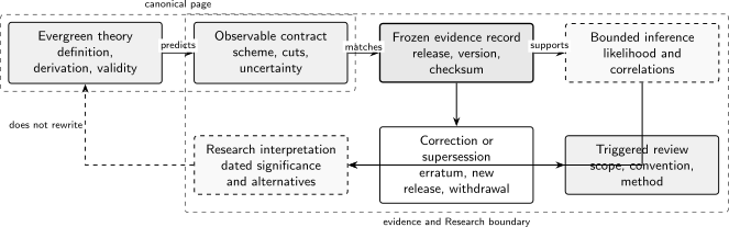
A new release or correction can supersede a Standard Model fit without changing the theory derivation. Every numerical conclusion therefore names the frozen evidence and likelihood versions; the diagram is schematic.

The joint likelihood is the fitted object

Let $d_a$ denote the data from input block $a$, $\boldsymbol\theta$ the parameters of interest, $\boldsymbol\eta_a$ block-specific nuisances, and $\boldsymbol\eta_s$ shared nuisances. If the primary observations are conditionally independent after common causes are represented, the joint likelihood can be written

$$L(\boldsymbol\theta,\boldsymbol\eta_s, \{\boldsymbol\eta_a\}) =\left[\prod_a L_a(d_a\mid\boldsymbol\theta, \boldsymbol\eta_s,\boldsymbol\eta_a) \right] L_{\rm aux}(a_{\rm aux}\mid \boldsymbol\eta_s,\{\boldsymbol\eta_a\}).$$

This product is justified by conditional independence, not by typography. If two inputs share events, an unfolded ancestor, control-region counts, or an auxiliary calibration, then one must build the relevant joint model, remove the overlap according to a predeclared rule, or omit one input. Duplicating a common auxiliary factor artificially tightens the nuisance and the parameters it controls.

The data block is meaningful only with its theory definition. A prediction may depend on pole and input schemes, perturbative scales, PDFs, hadronic matrix elements, matching coefficients, or EFT truncation. Sources representing the same missing-order or parametric direction must be correlated across blocks; sources with different physical causes should not be correlated merely because their quoted sizes are similar.

Generalized least squares as an exact check

For a linear Gaussian model

$$\mathbf y=A\boldsymbol\theta+\boldsymbol\epsilon, \qquad \boldsymbol\epsilon\sim N(\mathbf0,C),$$

with fixed positive-definite $C$, minimizing

$$\chi^2(\boldsymbol\theta) =(\mathbf y-A\boldsymbol\theta)^TC^{-1} (\mathbf y-A\boldsymbol\theta)$$

gives

$$\widehat{\boldsymbol\theta} =(A^TC^{-1}A)^{-1}A^TC^{-1}\mathbf y, \qquad \operatorname{Cov}(\widehat{\boldsymbol\theta}) =(A^TC^{-1}A)^{-1},$$

provided $A$ has full column rank in the metric defined by $C^{-1}$. This is a valuable analytic benchmark for a likelihood implementation.

Consider the exact two-bin fixture

$$\mathbf y=\begin{pmatrix}1\\2\end{pmatrix}, \qquad A=\begin{pmatrix}1\\1\end{pmatrix}, \qquad C=\begin{pmatrix}1&1/2\\1/2&4\end{pmatrix}.$$

Its determinant is $15/4>0$, and

$$C^{-1} =\begin{pmatrix} 16/15&-2/15\\ -2/15&4/15 \end{pmatrix}.$$

The numerator and denominator of the estimator are

$$A^TC^{-1}\mathbf y=\frac65, \qquad A^TC^{-1}A=\frac{16}{15},$$

so

$$\widehat\theta=\frac98, \qquad \chi^2_{\min}=\frac14.$$

The estimate is not the arithmetic mean: the correlated, unequal covariance changes the metric. Adding the two “pull squares” $(-1/8)^2/1+(7/8)^2/4$ does not reproduce $\chi^2_{\min}$ because it drops the off-diagonal term. A Cholesky factor $C=LL^T$ supplies whitened residuals $L^{-1}(\mathbf y-A\widehat\theta)$ whose Euclidean norm does reproduce the quadratic form.

Profiling and marginalization are different operations

Profiling maximizes the likelihood over nuisances at each parameter value:

$$L_{\rm prof}(\boldsymbol\theta) =L(\boldsymbol\theta, \widehat{\boldsymbol\eta}_{\boldsymbol\theta}).$$

Marginalization integrates them with a declared measure or prior density:

$$L_{\rm marg}(\boldsymbol\theta) =\int d\boldsymbol\eta\, L(\boldsymbol\theta,\boldsymbol\eta)\, \pi(\boldsymbol\eta).$$

They answer different inferential questions and generally have different shapes. An exact Gaussian fixture shows a special coincidence. Let

$$\chi^2(\theta,\eta) =(\theta+\eta-1)^2+\eta^2.$$

Completing the square gives

$$\chi^2 =2\left(\eta+\frac{\theta-1}{2}\right)^2 +\frac{(\theta-1)^2}{2}.$$

Therefore

$$\widehat\eta_\theta=\frac{1-\theta}{2}, \qquad \chi^2_{\rm prof}(\theta)=\frac{(\theta-1)^2}{2}.$$

With $L\propto e^{-\chi^2/2}$ and a flat integration measure in $\eta$,

$$L_{\rm marg}(\theta) =\sqrt\pi\, \exp\!\left[-\frac{(\theta-1)^2}{4}\right].$$

The profiled likelihood has the same $\theta$ dependence in this constant-width Gaussian example. That equality is not general: parameter-dependent curvature, boundaries, non-Gaussian auxiliary data, or a different integration measure change the marginalization factor. A published result must identify which operation and nuisance measure were used. Profile-likelihood asymptotics also require regularity and adequate sample size; small samples and boundaries call for simulation-based calibration Cowan et al. 2011, §§2–3, pp. 4–12.

Goodness of fit, pulls, and trials

In the fixed-covariance linear Gaussian model, if the mean model is correct and $A$ has rank $r$, then $\chi^2_{\min}$ follows a chi-square distribution with $n-r$ degrees of freedom. That statement can fail when:

• the covariance depends on fitted parameters or was estimated with material uncertainty;
• likelihood terms are non-Gaussian or counts are sparse;
• parameters lie on boundaries or are not identifiable under the null;
• the model is nonlinear over the supported region;
• data-dependent masks or regularization alter the statistic; or
• nuisance constraints are nonregular or duplicated.

In those cases, define the statistic and calibrate its sampling distribution with suitable pseudoexperiments or another justified method. The asymptotic formulas in Cowan et al. 2011, §§3–4, pp. 9–17 are approximations with explicit hypotheses, not labels that automatically turn a likelihood ratio into a significance.

A residual $y_i-\mu_i$ divided by its marginal standard deviation is not an independent test when entries are correlated. Useful diagnostics include whitened residuals, conditional residuals, nuisance pulls relative to their auxiliary constraints, and impacts obtained under a stated refit. Their collection remains correlated and should not be scanned as independent local significances.

Leave-one-block-out fits can reveal leverage or an inconsistent interface: refit after removing a predeclared block and compare predictions in that block. They do not by themselves assign a discovery probability, and repeatedly choosing the most discrepant omitted block introduces a trials problem.

For a search over masses, channels, operators, bins, or alternative masks, distinguish a local tail probability at a fixed hypothesis from a global probability for the predeclared search family. The family, scan resolution, and correlation structure must be fixed before calibration. A posterior selection of “interesting” trials cannot be repaired by quoting the local tail alone.

Freeze the fit contract

Component	Freeze before fitting	Check after fitting
Input identity	Dataset/table/workspace version, DOI or stable identifier, checksum and corrections	Every loaded byte and bin order matches the record
Observable and theory	Pole/fiducial definition, input and renormalization schemes, prediction version and accuracy	Benchmarks, dimensions, limits, and cross-scheme translation
Correlations	Covariance components or shared nuisance graph; auxiliary data included once	Symmetry/positivity, nuisance response, no duplicate constraint
Overlap	Event, control-region, unfolded-ancestor, and theory-input overlap rule	Product factorization is justified for retained blocks
Validity	Kinematic/EFT masks and parameter domains	Boundary hits and truncation stress tests are reported
Inference	Profiling or marginalization, statistic, degrees of freedom or calibration, trial family	Optimizer coverage, toy calibration, independent implementation
Lifecycle	Correction and supersession policy; output version	A corrected input creates a new result rather than silently replacing one

Publishing a statistical model rather than only its final contour preserves more of this structure and makes combinations and alternative parameterizations testable Cranmer et al. 2022, §§2–4, pp. 4–18.

Independent checks and failure modes

Positive definiteness. For an ordinary invertible Gaussian covariance, test symmetry, eigenvalues, and Cholesky factorization. A singular covariance may be legitimate for normalized data, but then the constrained subspace and generalized-inverse prescription must be explicit.

Duplicate input. Set up a table of event samples, controls, auxiliary measurements, and theory sources for every block. A repeated item needs one joint representation or a documented removal rule.

Analytic benchmark. Reproduce $\widehat\theta=9/8$ and $\chi^2_{\min}=1/4$ for the two-bin fixture. This tests matrix ordering, inversion, residual sign, and optimizer output independently.

Profile benchmark. Reproduce $\widehat\eta_\theta=(1-\theta)/2$ and the profiled curve above. Numerical profiling should agree over a grid, including points far enough from the optimum to exercise the implementation.

Coverage fixture. If $x\sim N(\theta,1)$ and the interval is predeclared as $[x-1,x+1]$, its exact coverage is

$$P_\theta(\theta\in[x-1,x+1]) =P(|x-\theta|\le1) =\operatorname{erf}\!\left(\frac1{\sqrt2}\right) =0.682689492\ldots.$$

A simulation or quadrature check should reproduce this value within its numerical tolerance. Choosing the interval or mask after observing $x$ invalidates that coverage statement.

Stability. Repeat the fit under predeclared leave-one-block-out, scheme, correlation, and validity variations. Explain the physical source of motion; do not convert the largest variation into an independent Gaussian error without a model.

Common pitfalls

Adding uncorrelated pulls. Off-diagonal covariance terms can raise or lower the joint discrepancy. Use the inverse covariance or full likelihood.

Profiling a nuisance twice. A covariance distilled from a profiled likelihood and the original auxiliary constraint are not independent inputs. Choose one faithful representation.

Treating profiling and marginalization as synonyms. They coincide in shape only in special Gaussian cases. State the operation, parameterization, and integration measure or auxiliary model.

Changing the data version or mask mid-fit. The resulting likelihood is not the one whose sampling properties were defined. Freeze versions and masks, then issue a new fit when an input changes.

Quoting a significance without a reference distribution. State the statistic, null, degrees of freedom or calibration, boundaries, and local/global trial definition.

Informal self-check

Derive the generalized least-squares estimate and minimum chi-square for the two-bin fixture above without numerical minimization.

Solution

Using the displayed inverse,

$$C^{-1}\mathbf y =\begin{pmatrix}4/5\\2/5\end{pmatrix}, \qquad C^{-1}A =\begin{pmatrix}14/15\\2/15\end{pmatrix}.$$

Thus $A^TC^{-1}\mathbf y=6/5$ and $A^TC^{-1}A=16/15$, giving $\widehat\theta=(6/5)/(16/15)=9/8$. The residual is $(-1/8,7/8)^T$; substitution into $r^TC^{-1}r$ gives $1/4$.

Handoffs

• Return to collider measurements and likelihood provenance if any input lacks exact identity, nuisance semantics, or an overlap rule.
• Return to electroweak precision observables for input-scheme and sector-covariance construction.
• Return to Higgs precision and coupling inference for width, response, and EFT assumptions in Higgs blocks.
• Reproduce the analytic covariance, nuisance, and coverage fixtures before applying the workflow to released inputs.

References

• Cowan, Glen, Kyle Cranmer, Eilam Gross, and Ofer Vitells. “Asymptotic Formulae for Likelihood-Based Tests of New Physics.” European Physical Journal C 71 (2011) 1554. DOI · Open PDF
• Cranmer, Kyle, et al. “Publishing Statistical Models: Getting the Most out of Particle Physics Experiments.” SciPost Physics 12 (2022) 037. DOI · Open PDF