

Dynamical Gauge Fields and Matter
A gauge connection becomes a dynamical quantum field when the action contains a gauge-field kinetic term and the functional integral—or canonical phase space—includes that connection among the variables. Charged matter then couples through the same covariant derivative that defines parallel transport. The result is not merely a collection of vector fields: gauge redundancy produces a Gauss constraint, removes unphysical polarizations, and forces charged observables to be dressed.
Required background. Gauge fields, redundancy, and observable content supplies connections, gauge transformations, and the distinction between redundancy and physical symmetry.
Helpful background. Gauging continuous and finite symmetries distinguishes a background connection from a field that is integrated over.
The map below places the dynamical starting point developed on this page inside the diagnostic chain used throughout the chapter. Read it vertically: a regime label becomes meaningful only after the matter content and global form have fixed which probes are genuine and which charges can be screened.
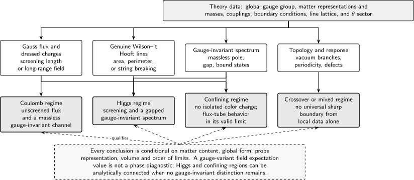
Gauge-regime diagnostic map. Spectra and long-range response, screening classes, genuine line operators, and topological sectors supply complementary information; no single arrow is a universal order parameter. Every branch is qualified by the gauge group’s global form and the dynamical matter content. The diagram is schematic.
Gauge–matter action and convention specification
Section titled “Gauge–matter action and convention specification”Take a compact gauge group with Lie algebra generators represented by Hermitian matrices on a Dirac field . Write
and
The entries below are the minimum data needed before comparing formulas across sources or models.
| Item | Convention used here | Why it matters |
|---|---|---|
| Spacetime | Four-dimensional Lorentzian spacetime, metric | Fixes signs in the kinetic and Hamiltonian terms |
| Generators | , | Fixes the structure constants and group factors |
| Fundamental trace | for | Fixes the standard beta-function normalization |
| Local gauge field | Fixes the sign in and the matter source | |
| Global gauge group | Must be declared separately from its Lie algebra | Determines allowed bundles, genuine lines, and charge sectors |
| Boundary data | Fixed at the boundary, fixed normal flux, or stated falloff | Determines whether the variational principle and charges are well defined |
For a local transformation in the matter representation,
These laws make . Their derivation from parallel transport, including the sign convention, is given in Schwartz 2014, §25.2.2, pp. 490–493.
The minimal Yang–Mills–Dirac action is
A complex scalar in a representation can be included by adding . Gauge invariance restricts to invariant combinations, but does not require a gauge-variant expectation value to be an observable.
Two separate choices make dynamical. First, the term gives it local propagation and a canonical momentum. Second, the quantum theory integrates over modulo gauge transformations. A source field held fixed while matter is quantized is a background gauge field, even if it has spacetime dependence.
Field equations and the boundary term
Section titled “Field equations and the boundary term”The non-Abelian variation is organized by
After one covariant integration by parts,
where, for the sign convention above,
Thus
One could instead call the matter current and write ; the physics is identical, but the definition must accompany the equation. The gauge-field equations and their covariant current identity are developed in Weinberg 1996, §15.3, pp. 12–14.
The displayed surface term is not optional bookkeeping. It vanishes, for example, when the appropriate components of are fixed on , when normal flux is fixed after adding the corresponding boundary term, or under sufficiently rapid falloff at spatial infinity. Different admissible boundary conditions can leave different boundary symmetries and charges. An action without that choice is not yet a complete variational problem.
Taking a covariant divergence of the gauge-field equation gives on the matter equations. This is a consistency identity tied to gauge covariance; it is not an additional independent evolution equation.
Gauss law and physical degrees of freedom
Section titled “Gauss law and physical degrees of freedom”On a constant-time slice define
The equation contains no second time derivative of :
Canonically, the momentum conjugate to vanishes, , and preservation of that primary constraint gives . Both are first-class constraints. On physical states the quantum condition is
for gauge transformations treated as redundancies. Transformations that approach a nontrivial value at a boundary can instead act on physical charge sectors; which transformations are quotiented is therefore part of the boundary specification. The canonical constraint analysis is given in Weinberg 1996, §15.4, pp. 14–17.
The counting makes the physical content concrete. Per Lie-algebra generator, begins with eight phase-space variables. The two first-class constraints remove four phase-space dimensions, leaving four: two configuration-space polarizations for a massless gauge boson. Gauge fixing selects one representative of each orbit; it does not restore the discarded polarizations as particles.
Charged matter fields are not, by themselves, gauge-invariant operators. In Abelian language one possible equal-time dressing is
Under gauge transformations that vanish at infinity, the exponential cancels the transformation of . Different describe different physical field profiles—for example a Coulombic cloud or a thin string—not different gauges of the same state. Non-Abelian dressings require path ordering and have additional global and Gribov-related qualifications.
Independent checks and limits
Section titled “Independent checks and limits”Several checks catch most convention errors.
- Gauge covariance: transforms by conjugation, so and the matter kinetic term are invariant.
- Abelian limit: setting reduces the equations to Maxwell theory with the declared sign of the source.
- Energy: after imposing the constraint, the pure-gauge Hamiltonian density contains , so propagating modes have positive energy.
- Dimensions: in four dimensions , , and ; every displayed bulk term has mass dimension four.
- Weak-coupling limit: the non-Abelian self-interactions vanish order by order as , but the global form and allowed probes are not erased by that perturbative limit.
The two-polarization count is perturbative around a background for which the usual local analysis applies. In a Higgs regime the gauge-invariant spectrum can contain massive spin-one states; in a confining regime no asymptotic colored gauge boson need exist. The constraint and gauge redundancy persist in both cases.
Common pitfalls
Section titled “Common pitfalls”Equating “gauged” with “dynamical.” Introducing a background connection makes a symmetry local in the source-coupled description. It becomes a quantum gauge field only after a kinetic term and integration over gauge configurations are specified.
Calling gauge charge an ordinary local charge. Gauss law ties charge to flux and to boundary behavior. A physical charged operator must carry a dressing or end on a boundary or defect that absorbs its gauge variation.
Dropping the surface term. Bulk Euler–Lagrange equations do not define the theory at a boundary. State the boundary condition or add the boundary action that makes the chosen data variationally admissible.
Using a gauge-fixed field as a phase diagnostic. A convenient gauge may expose perturbative masses, but phase statements require gauge-invariant spectra, forces, defects, or symmetry realization.
Continue with Charges, screening, and long-range forces to turn the local constraint into a large-distance test.
References
Section titled “References”Original QFT.org content:CC BY 4.0, unless an item supplies different terms. Third-party material retains its own terms.