

Higgs Interactions, Production, Decay, and Pole Observables
A defensible Higgs prediction begins with a renormalized electroweak parameter set and a complex-pole definition, builds complete production and decay amplitudes, and only then maps them to inclusive, fiducial, or pseudo-observables with correlated uncertainties. This chain prevents an isolated coupling, diagram, branching fraction, or line-shape parameter from being mistaken for a directly measured quantity.
Required background. Electroweak renormalization and input schemes supplies the parameters, tadpole prescription, pole conventions, and perturbative order. Unstable-particle observables and resonance approximations supplies the analytic pole expansion and the conditions for resonance factorization.
Helpful background. Higgs self-interactions and the scalar potential supplies the distinction between a renormalized self-coupling and a multi-Higgs observable.
The map below separates the evergreen amplitude and scheme relations from the evidence layer. Higgs self-couplings, symmetry breaking, Yukawa couplings, high-energy cancellations, and renormalized pole amplitudes meet at a precisely declared observable before any dated measurement or combination is interpreted.
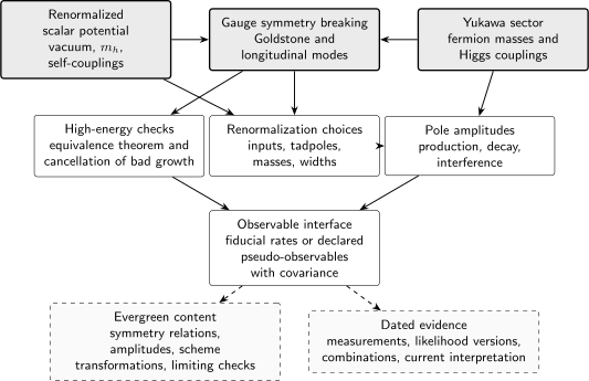
Higgs predictions require compatible symmetry, renormalization, pole, and observable definitions. Measurements, likelihood versions, combinations, and current interpretations remain in dated evidence records; the diagram is schematic.
Couplings and production mechanisms
Section titled “Couplings and production mechanisms”For , , and
the tree-level terms linear in the radial field include
These vertices seed the standard production classes, but a prediction also requires QCD and electroweak radiation, parton distributions for hadronic beams, unstable-particle treatment, and a measurement definition. The interactions follow from the Higgs kinetic and Yukawa terms as developed in Schwartz 2014, §§29.1 and 29.3, pp. 584–599.
| Production class | Amplitude-level origin | Definition and consistency questions |
|---|---|---|
| Gluon fusion, | colored-particle loops, with quark Yukawa couplings in the minimal model | quark-mass scheme, exact-mass versus effective description, QCD order, PDFs, jet-bin definition |
| Vector-boson fusion, | two electroweak quark currents joined by the interaction | fiducial VBF definition, interference with other amplitudes, electroweak and nonfactorizable corrections |
| Associated production | an electroweak current produces an off-shell , or a loop-induced partonic channel, followed by | separate partonic channels and -decay treatment; avoid folding a loop-induced component into a different perturbative order |
| Heavy-quark associated production | , single-top–Higgs, or bottom-associated amplitudes probe Yukawa interactions | heavy-flavor scheme, mass definition, interference among gauge and Yukawa diagrams, decay and acceptance treatment |
| Multi-Higgs production | self-interaction diagrams interfere with boxes, Yukawa, gauge, and possible contact terms | parameter basis, complete gauge-invariant amplitude, resonant substructure, and correlated variations |
This is a mechanism classification, not a ranking by current rate or sensitivity. The LHC Higgs Cross Section Working Group organizes production, decay, off-shell effects, fiducial quantities, and pseudo-observables in this way in de Florian et al. 2017, Parts I and III.
At fixed order, a label such as “VBF” or “” can refer to a calculational signal definition rather than an exactly isolated set of observed events. The page or dataset using the label must state the partonic channels, perturbative orders, phase-space cuts, overlap removal, and interference retained.
Decay amplitudes and branching fractions
Section titled “Decay amplitudes and branching fractions”The same renormalized couplings generate several structurally different decay classes.
| Decay class | Leading structure | Required qualifications |
|---|---|---|
| Yukawa coupling | fermion-mass and Yukawa scheme, QCD/QED radiation, infrared-safe final-state definition | |
| or , followed by decays | coupling and electroweak currents | off-shell vector propagators when required, spin correlations, identical-particle interference, fiducial final state |
| colored-particle loop | QCD order, mass dependence, effective-theory validity, inclusive radiation convention | |
| or | coherent sum of charged-particle loops | relative phases and interference, electroweak inputs, -decay and photon isolation definitions |
| multi-scalar, invisible, or unobserved channels | only when allowed by the declared spectrum and parameterization | thresholds, new-state assumptions, total-width closure, and model dependence |
For a mutually exclusive and complete set of decay definitions,
Completeness is an assumption to check, not a notational fact. If channels are omitted or an unobserved component is allowed, the total width needs an explicit additional parameter. Likewise, partial widths are theory-defined pseudo-observables only after soft radiation, off-shell daughter states, and phase-space conventions are fixed.
Pole expansion and pseudo-observables
Section titled “Pole expansion and pseudo-observables”Let be the invariant carried by a scalar resonance. Near an isolated simple pole, an amplitude can be organized as
The pole , its consistently defined residue, and the full amplitude are gauge-independent; selected resonant diagrams away from the pole need not be. Analytic pole expansion provides the clean separation between resonance parameters and regular background Stuart 1991, pp. 113–119.
For a single nondegenerate state, the residue factorizes into production and decay factors after external-state conventions are fixed. This motivates pole pseudo-observables such as effective residues and partial widths. They remain derived quantities: an experiment observes distributions of stable final states, while theory and a likelihood map those distributions to the pole parameterization.
Near a narrow, isolated resonance one often uses
This narrow-width approximation requires all of the following:
- is small over the relevant resolution scale;
- production, decay, luminosity, and phase-space factors vary slowly across the pole;
- cuts and bin boundaries do not strongly distort the resonance region;
- interference with is negligible or corrected;
- nearby thresholds or resonances do not spoil the single-pole expansion.
If any condition fails, compute the stable-final-state amplitude including the pole and continuum together. An off-shell distribution can constrain the same couplings that appear on shell, but a conversion into a total-width statement is model-dependent unless the relation between on-shell and off-shell amplitudes is specified.
Inclusive, fiducial, and template observables
Section titled “Inclusive, fiducial, and template observables”An inclusive cross section integrates a defined final state over a broad phase space. A fiducial cross section instead includes a particle-level measurement function :
This schematic equation records the ingredients that must agree between theory and measurement: incoming-state convention, PDFs, scales, stable final state, radiation and recombination rules, and fiducial cuts. Detector unfolding and migration introduce another response model and covariance.
Template cross sections partition a fiducial region into bins designed to retain production or kinematic information. Their virtue is a shorter extrapolation than a total inclusive rate; their limitation is dependence on bin definitions, migration modeling, and the theory used to connect bins to couplings. The working-group treatment of fiducial and simplified-template observables is given in de Florian et al. 2017, Part III, chs. 2–3.
Do not combine an inclusive theory prediction with a fiducial measured number by applying an acceptance from a different model without propagating the resulting uncertainty. Also do not call a fitted signal-strength parameter a coupling until the production, decay, width, and unseen-channel assumptions have been written down.
Correlated prediction uncertainties
Section titled “Correlated prediction uncertainties”For small variations of the partial widths,
Thus a change in one partial width moves every branching fraction through the shared denominator. If is the partial-width covariance, define
Independent quadrature of branching-fraction errors discards this anticorrelation. The same issue appears across production bins when a common scale, PDF eigenvector, coupling, shower model, or luminosity nuisance moves several bins coherently.
A complete theory-uncertainty statement separates and correlates, as applicable:
- missing higher orders in QCD and electroweak expansions, including the scale-variation prescription;
- PDFs, , running masses, and other parametric inputs;
- heavy-mass expansions, matching, resummation, and threshold choices;
- pole, narrow-width, interference, and off-shell approximations;
- parton shower, hadronization, underlying-event, and acceptance modeling;
- numerical integration, interpolation, and finite simulation samples.
Scale variation probes sensitivity to uncalculated terms; it is not a probability distribution by itself. Scheme and matching variations can supply complementary diagnostics, but overlapping variations should not be counted twice.
Reproducible evidence interface
Section titled “Reproducible evidence interface”Before a numerical prediction or inference is compared, record
| Layer | Minimum information |
|---|---|
| Physics state | model and parameter basis; Higgs pole, residue, and total-width conventions |
| Calculation | process and decay definition; perturbative orders; scales; PDFs; masses; electroweak input and tadpole schemes |
| Approximation | effective operators, resummation, narrow-width or off-shell treatment, interference, validity tests |
| Measurement | collision system and energy; dataset period; stable final state; fiducial bins; unfolding or response model |
| Uncertainty | named sources, correlations, covariance or nuisance implementation, missing-order prescription |
| Provenance | collaboration or author, release identifier, version, publication date, files or tables used, corrections and supersession |
| Inference | likelihood or test statistic, priors if any, parameter ranges, fixed assumptions, and goodness-of-fit diagnostics |
Current masses, widths, rates, limits, combinations, production rankings, and compatibility statements are time-dependent evidence claims. They should be stated only with a named release or calculation, its dataset period and version, a dated evidence cutoff, and the likelihood or covariance needed to reproduce the inference. No such current numerical or status claim is made on this durable methods page.
Checks and failure modes
Section titled “Checks and failure modes”Pole check. Vary gauge-fixing parameters in the complete calculation. The complex pole and physical stable-state observable must remain unchanged through the computed order.
Factorization check. Compare the full line shape with the narrow-width result under the actual cuts. A small alone does not control interference or acceptance variation.
Closure check. Verify whether the fitted branching fractions sum to one by assumption. If an unseen width is allowed, include it explicitly in and the covariance.
Coupling check. Change one renormalized coupling only within a gauge-consistent parameterization. Rescaling a selected diagram can violate Ward identities and misstate interference.
Provenance check. A table copied from a later theory release may use different PDFs, masses, or uncertainty correlations from the likelihood. Match versions before combining them.
Common pitfalls
Section titled “Common pitfalls”Equating a production label with an observed event category. Categories have migrations and contributions from several mechanisms. Use a response matrix or a documented purity model.
Turning an off-shell tail directly into a width. The inference requires assumptions relating on-shell residues, off-shell amplitudes, and any new continuum contributions.
Adding theory uncertainties as independent percentages. Common inputs and shared denominators create correlations. Propagate a covariance or explicit nuisance model.
Handoff
Section titled “Handoff”A reusable Higgs prediction or inference passes
Use this object in Precision Standard Model. Time-dependent experimental combinations and reinterpretations belong to Research: EFT and Standard Model Tests, with their dated evidence and likelihood artifacts attached.
References
Section titled “References”- de Florian, D., C. Grojean, F. Maltoni, C. Mariotti, A. Nikitenko, M. Pieri, P. Savard, M. Schumacher, R. Tanaka, et al., eds. Handbook of LHC Higgs Cross Sections: 4. Deciphering the Nature of the Higgs Sector. CERN Yellow Reports: Monographs 2/2017, CERN-2017-002-M, 2017, pp. 1–869. DOI. Open PDF.
- Schwartz, Matthew D. Quantum Field Theory and the Standard Model. Cambridge University Press, 2014, §§29.1 and 29.3, pp. 584–599. DOI.
- Stuart, Robin G. “Gauge Invariance, Analyticity and Physical Observables at the Resonance.” Physics Letters B 262, no. 1 (1991): 113–119. DOI.
Original QFT.org content:CC BY 4.0, unless an item supplies different terms. Third-party material retains its own terms.